21. Multiple Integrals in Curvilinear Coordinates
d. Integrating in 2D Curvilinear Coordinates
5. Diamond Shaped Examples
Below is an example of using curvilinear coordinates to compute an integral over a “diamond shaped” region.
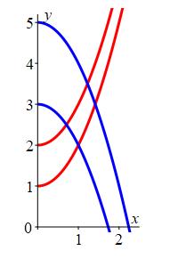
Compute the integral \(\displaystyle \iint xy\,dA\) over the
diamond shaped region, \(R\), in the first quadrant bounded by
\(y=1+x^2\) and \(y=2+x^2\) in red
and
\(y=3-x^2\) and \(y=5-x^2\) in blue.
We look at the boundary curves to determine useful coordinates (\(u\) and \(v\)) for this problem. The first two curves, \(y=1+x^2\) and \(y=2+x^2\), can be written as: \[ y-x^2=1 \quad \text{and} \quad y-x^2=2 \] If we let \(u=y-x^2\), then the bounds for \(u\) become \[ u=1 \quad \text{and} \quad u=2 \] Similarly, the other two curves, \(y=3-x^2\) and \(y=5-x^2\), can be written as: \[ y+x^2=3 \quad \text{and} \quad y+x^2=5 \] If we let \(v=y+x^2\), then the bounds for \(v\) become \[ v=3 \quad \text{and} \quad v=5 \] Summarizing, \[ u=y-x^2 \qquad \text{and} \qquad v=y+x^2 \qquad \text{(*)} \] Next we need to find the Jacobian \(J=\left|\dfrac{\partial(x,y)}{\partial(u,v)}\right|\). This requires us to know \(x\) and \(y\) as functions of \(u\) and \(v\), but unfortunately, we know \(u\) and \(v\) as functions of \(x\) and \(y\). So we need to solve (*) for \(x\) and \(y\). There are two way to do this:
First, we can solve one equation for one variable and plug into the other. For example, if we solve the first equation for \(y=u+x^2\) then the second equation becomes \(v=u+2x^2\) or \(x^2=\dfrac{v-u}{2}\) or \(x=\sqrt{\dfrac{v-u}{2}}\). We plug this back into \(y=u+x^2\) to get \(y=u+\dfrac{v-u}{2}=\dfrac{v+u}{2}\).
Alternatively, we can add and subtract the equations. If we add, we get \(u+v=2y\) or \(y=\dfrac{v+u}{2}\). If we subtract, we get \(u-v=-2x^2\) or \(x=\sqrt{\dfrac{v-u}{2}}\).
By either method we get: (It's beneficial to split off the \(\sqrt{2}\) in the denominator since we are going to differentiate.) \[ x=\sqrt{\dfrac{v-u}{2}}=\dfrac{\sqrt{v-u}}{\sqrt{2}} \qquad \text{and} \qquad y=\dfrac{v+u}{2} \qquad \text{(**)} \]
Now we can compute the Jacobian: \[\begin{aligned} J&=\left|\begin{vmatrix} \dfrac{\partial x}{\partial u} & \dfrac{\partial y}{\partial u} \\[8pt] \dfrac{\partial x}{\partial v} & \dfrac{\partial y}{\partial v} \end{vmatrix}\right| =\left|\begin{vmatrix} \dfrac{-1}{2\sqrt{2}\sqrt{v-u}} & \dfrac{1}{2} \\[8pt] \dfrac{1}{2\sqrt{2}\sqrt{v-u}} & \dfrac{1}{2} \end{vmatrix}\right| \\ &=\left|\dfrac{-1}{4\sqrt{2}\sqrt{v-u}}-\,\dfrac{1}{4\sqrt{2}\sqrt{v-u}}\right| =\left|\dfrac{-1}{2\sqrt{2}\sqrt{v-u}}\right|=\dfrac{1}{2\sqrt{2}\sqrt{v-u}} \end{aligned}\] We dropped the minus sign because a square root is always posiitve. The last thing we need is the integrand: \[ xy=\dfrac{\sqrt{v-u}(v+u)}{2\sqrt{2}} \] We can now compute the integral: \[\begin{aligned} I&=\iint xy\,dA =\iint xy \,J\,du\,dv \\ &=\int_3^5\int_1^2 \dfrac{\sqrt{v-u}(v+u)}{2\sqrt{2}}\dfrac{1}{2\sqrt{2}\sqrt{v-u}}\,du\,dv \\ &=\dfrac{1}{8}\int_3^5\int_1^2 (v+u)\,du\,dv \\ &=\dfrac{1}{8}\left[\dfrac{v^2}{2}\dfrac{}{}\right]_3^5\left[u\dfrac{}{}\right]_1^2 +\dfrac{1}{8}\left[v\dfrac{}{}\right]_3^5\left[\dfrac{u^2}{2}\right]_1^2 \\ &=\dfrac{1}{8}\left(\dfrac{25-9}{2}(1)+(2)\dfrac{4-1}{2}\right) =\dfrac{1}{8}\left(8+3\right)=\dfrac{11}{8} \end{aligned}\]
Notice how easy this integral was once we had the coordinate system and the Jacobian. Imagine doing it in rectangular coordinates. We would have to find all the intersection points, break the integral into \(3\) regions and integrate with bounds which were quadratic.
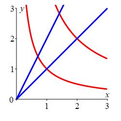
Find the area of the diamond shaped region bounded by \(y=\dfrac{1}{x}\) and \(y=\dfrac{4}{x}\) in red and \(y=x\) and \(y=2x\) in blue. To do this, find a curvilinear coordinate system for which the \(4\) boundary curves are specified by constant values of the \(2\) coordinates. Then find the Jacobian factor and the area.
Define \(u\) and \(v\) in terms of \(x\) and \(y\) so that the boundaries become constant values of \(u\) and \(v\). Then solve for \(x\) and \(y\) as functions of \(u\) and \(v\) so you can compute the Jacobian.
The coordinates may be taken as \(u=xy\) and \(v=\dfrac{y}{x}\).
Then the boundaries are \(u=1\), \(u=4\), \(v=1\) and \(v=2\).
The coordinate system is \(x=\sqrt{\dfrac{u}{v}}\) and \(y=\sqrt{uv}\).
The Jacobian factor is \(J=\dfrac{1}{2v}\).
The area is \(\dfrac{3}{2}\ln2\).
We look at the boundary curves to determine useful coordinates (\(u\) and \(v\)) for this problem. The first two curves, \(y=\dfrac{1}{x}\) and \(y=\dfrac{4}{x}\), can be written as: \[ xy=1 \quad \text{and} \quad xy=4 \] If we let \(u=xy\), then the bounds for \(u\) become \[ u=1 \quad \text{and} \quad u=4 \] Similarly, the other two curves, \(y=x\) and \(y=2x\), can be written as: \[ \dfrac{y}{x}=1 \quad \text{and} \quad \dfrac{y}{x}=2 \] If we let \(v=\dfrac{y}{x}\), then the bounds for \(v\) become \[ v=1 \quad \text{and} \quad v=2 \] Summarizing, \[ u=xy \quad \text{and} \quad v=\dfrac{y}{x} \qquad \qquad (*) \] However, to compute the Jacobian \(J=\left|\dfrac{\partial(x,y)}{\partial(u,v)}\right|\). we need to know \(x\) and \(y\) as functions of \(u\) and \(v\). To find \(x\) and \(y\), we multiply and divide the equations. If we multiply (*), we get \(uv=xy\dfrac{y}{x}=y^2\) or \(y=\sqrt{uv}\). If we divide (*), we get \(\dfrac{u}{v}=xy\dfrac{x}{y}=x^2\) or \(x=\sqrt{\dfrac{u}{v}}\). It's beneficial to write these formulas with fractional powers since we are going to differentiate. \[ x=\sqrt{\dfrac{u}{v}}=u^{1/2}v^{-1/2} \qquad \text{and} \qquad y=\sqrt{uv}=u^{1/2}v^{1/2} \]
Now we can compute the Jacobian: \[\begin{aligned} J&=\left|\begin{vmatrix} \dfrac{\partial x}{\partial u} & \dfrac{\partial y}{\partial u} \\[8pt] \dfrac{\partial x}{\partial v} & \dfrac{\partial y}{\partial v} \end{vmatrix}\right| =\left|\begin{vmatrix} \dfrac{1}{2}u^{-1/2}v^{-1/2} & \dfrac{1}{2}u^{-1/2}v^{1/2} \\[8pt] \dfrac{-1}{2}u^{1/2}v^{-3/2} & \dfrac{1}{2}u^{1/2}v^{-1/2} \end{vmatrix}\right| \\ &=\left|\dfrac{1}{4}v^{-1}-\,\dfrac{-1}{4}v^{-1}\right| =\left|\dfrac{1}{2v}\right|=\dfrac{1}{2v} \end{aligned}\] We dropped the absolute value because \(v\) is posiitve. So the area is: \[\begin{aligned} A&=\iint_R 1\,dA=\iint_R J\,du\,dv =\int_1^2\int_1^4 \dfrac{1}{2v}\,du\,dv \\ &=\dfrac{1}{2}\int_1^4 1\,du\int_1^2 \dfrac{1}{v}\,dv =\dfrac{1}{2}\left[\rule{0pt}{10pt}u\right]_1^4 \left[\rule{0pt}{10pt}\ln|v|\right]_1^2 \\ &=\dfrac{1}{2}(4-1)\ln2=\dfrac{3}{2}\ln2 \approx1.04 \end{aligned}\]
The next page on applications of 2D curvilinear coordinates has lots of additional examples and exercises.
Heading
Placeholder text: Lorem ipsum Lorem ipsum Lorem ipsum Lorem ipsum Lorem ipsum Lorem ipsum Lorem ipsum Lorem ipsum Lorem ipsum Lorem ipsum Lorem ipsum Lorem ipsum Lorem ipsum Lorem ipsum Lorem ipsum Lorem ipsum Lorem ipsum Lorem ipsum Lorem ipsum Lorem ipsum Lorem ipsum Lorem ipsum Lorem ipsum Lorem ipsum Lorem ipsum